In 1610, shortly after viewing the sun with his ‘new telescope’, Galileo Galilei made the first European observations of sunspots. Daily observations were started at the Zurich Observatory in 1749 and with the addition of other observatories continuous observations were obtained starting in 1849.Early records of sunspots indicate that the Sun went through a period of inactivity in the late 17th century. Very few sunspots were seen on the Sun from about 1645 to 1715. Although the observations were not as extensive as in later years, the Sun was in fact well observed during this time and this lack of sunspots is well documented. This period of solar inactivity also corresponds to a climatic period called the “Little Ice Age” when rivers that are normally ice-free, froze and snow fields remained year-round at lower altitudes. There is evidence that the Sun has had similar periods of inactivity in the more distant past. The connection between solar activity and terrestrial climate is an area of on-going research.
The Royal Greenwich Observatory has obtained detailed observations of sunspots since 1874. These observations include information on the sizes and positions of sunspots as well as their numbers. These data show that sunspots do not appear at random over the surface of the sun but are concentrated in two latitude bands on either side of the equator. A butterfly diagram (updated monthly) showing the positions of the spots for each rotation of the sun since May 1874 shows that these bands first form at mid-latitudes, widen, and then move toward the equator as each cycle progresses. The cycles overlap at the time of sunspot cycle minimum with old cycle spots near the equator and new cycle spots at high latitudes.
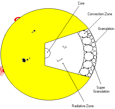
The photosphere is the visible surface of the Sun that we can observe. Since the Sun is a ball of gas, this is not a solid surface but is actually a layer about 100 km thick (very, very, thin compared to the 700,000 km radius of the Sun). When we look at the centre of the disk of the Sun we look ‘straight in’ and see somewhat hotter and brighter regions. When we look at the limb, ‘or edge’ of the solar disk we see light that has taken a slanting path through this layer and we only see through the upper, cooler and dimmer regions. This explains the “limb darkening” that appears as a darkening of the solar disk near the limb.
The Sun rotates on its axis once in about 27 days. This rotation was first detected by observing the motion of sunspots in the photosphere. The Sun’s rotation axis is tilted by about 7.25 degrees from the axis of the Earth’s orbit so we see more of the Sun’s North Pole in September of each year and more of its south pole in March.
A number of features can be observed in the photosphere with a simple telescope (along with a good filter to reduce the intensity of sunlight to safely observable levels). These features include the dark sunspots, the bright faculae, and granulation.
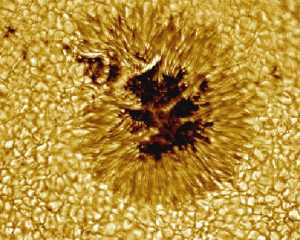
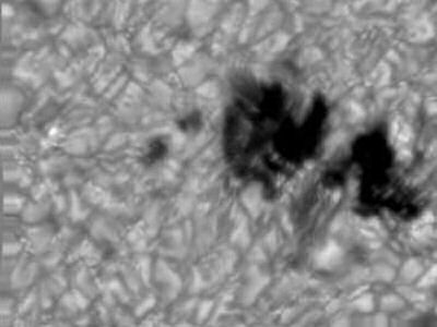
Sunspots
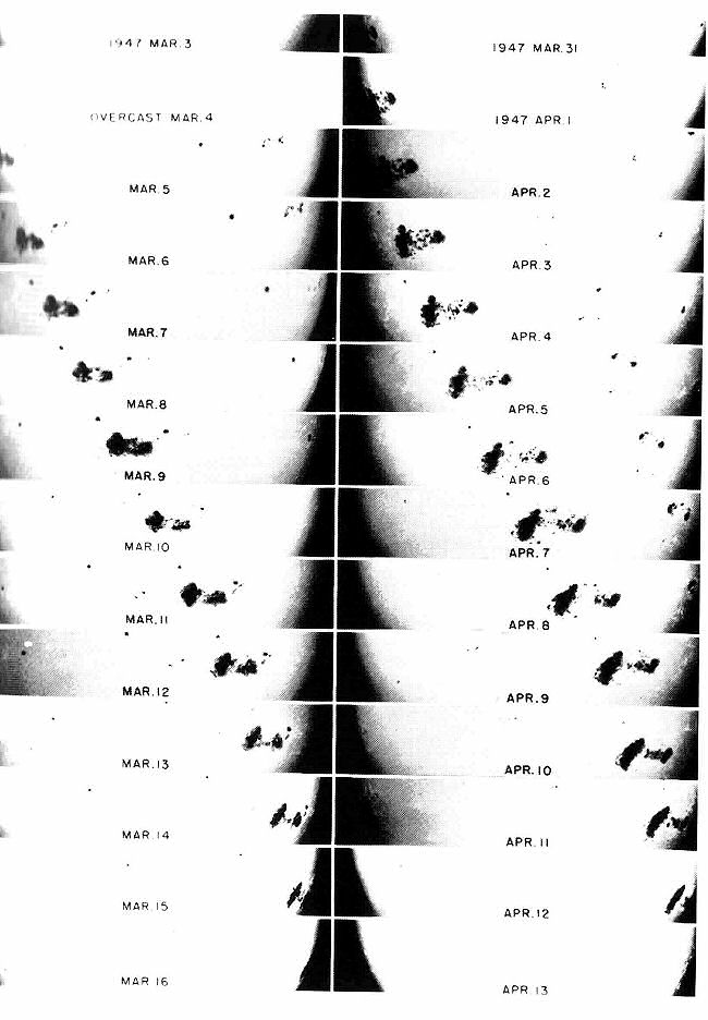
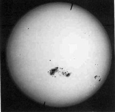
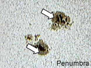
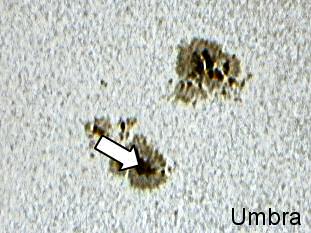
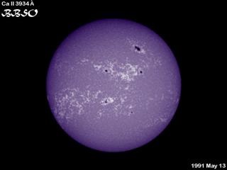
Sunspots appear as dark spots on the visible surface of the Sun. Temperatures in the dark centres of sunspots drop to about 3700 K (compared to 5700 K for the surrounding photosphere). They typically last for several days, although very large ones may live for several weeks. Sunspots are magnetic regions on the Sun with magnetic field strengths thousands of times stronger than the Earth’s magnetic field. Sunspots usually come in groups with two sets of spots. One set will have positive or north magnetic field while the other set will have negative or south magnetic field. The field is strongest in the darker parts of the sunspots – the umbra. The field is weaker and more horizontal in the lighter part – the penumbra. The largest sunspot ever recorded was visible in March and April 1947 and covered an area of over 7,000 million square miles; about a hundred Earths could be fitted into this area!
The sunspot number is calculated by first counting the number of sunspot groups and then the number of individual sunspots. The “sunspot number” is then given by the sum of the number of individual sunspots and ten times the number of groups. Since most sunspot groups have, on average, about ten spots, this formula for counting sunspots gives reliable numbers even when the observing conditions are less than ideal and small spots are hard to see. Monthly averages show that the number of sunspots visible on the sun waxes and wanes with an approximate 11-year cycle. It is interesting to recall that it was Samuel Heinrich Schwabe ( 1789– 1875), a German apothecary and amateur astronomer that discovered the 11-year cycle. In the hope of discovering a new planet between Mercury and the Sun, he made daily observations and tallies of sunspots. In 1843, after 17 years of sunspot counts, he noted a periodicity of 10 or 11 years in their totals. Julius Schmidt and Rudolf Wolf supported this periodicity while others remained sceptical. Only when other independent observations made by Wolf, Sabine, Gautier and J. von Lamont supported the sunspot cycle and variations in the Earth’s magnetic field with an 11-year frequency, did Schwabe receive wide support. Before that time (1826 – 51) no such periodicity was even suspected. The RAS Library at Burlington House, London, keeps 31 volumes with his observational notes covering the years 1825 to 1867.
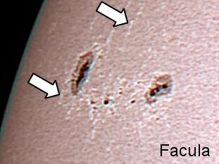
Faculae
Faculae are bright areas that are usually most easily seen near the limb, or edge, of the solar disk. These are also magnetic areas but the magnetic field is concentrated in much smaller bundles than in sunspots. While the sunspots tend to make the Sun look darker, the faculae make it look brighter. During a sunspot cycle the faculae actually win out over the sunspots and make the Sun appear slightly (about 0.1%) brighter at sunspot maximum than at sunspot minimum.
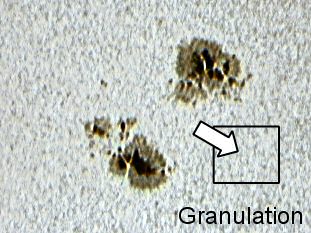
Granulation
Granules are small (about 1000 km across) cellular features that cover the entire Sun except for those areas covered by sunspots. These features are the tops of convection cells where hot fluid rises up from the interior in the bright areas, spreads out across the surface, cools and then sinks inward along the dark lanes. Individual granules last for only about 20 minutes. The granulation pattern is continually evolving as old granules are pushed aside by newly emerging ones. The flow within the granules can reach supersonic speeds of more than 7 km/s (15,000 mph) and produce sonic “booms” and other noise that generates waves on the Sun’s surface.
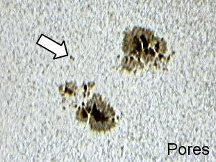
Pores
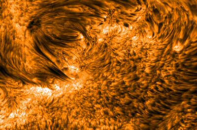
Solar pores are small sunspots that lack a penumbral structure. Because they are part of the early stage of sunspot evolution, they are important in understanding the mechanism of small-scale flux emergence on the surface of the Sun. The magnetic field lines in pores are almost vertical, however, the lines of force in sunspot penumbrae are highly inclined. Studying the evolution of pores can lead to a better understanding of the interaction between magnetic fields and the surrounding convective motions. In order to study the fine structures in and around pores and sunspots, high spatial, temporal, and spectral resolution observations are needed. The disturbing effect of the Earth’s atmosphere limits the resolution that we can obtain even when using large telescopes.
Super Granules
Super granules are much larger versions of granules (about 35,000 km across) but are best seen in measurements of the “Doppler shift” where light from material moving toward us is shifted to the blue while light from material moving away from us is shifted to the red. These features also cover the entire Sun and are continually evolving. Individual super granules last for a day or two and have flow speeds of about 0.5 km/s (1000 mph). The fluid flows observed in super granules carry magnetic field bundles to the edges of the cells where they produce the chromospheric network.
The Chromospheric Network
The chromospheric network is a web-like pattern most easily seen in the emissions of the red line of hydrogen (H-alpha) and the ultraviolet line of calcium (Ca II K – from calcium atoms with one electron removed). The network outlines the super granule cells and is due to the presence of bundles of magnetic field lines that are concentrated there by the fluid motions in the super granules.
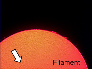
Filaments and Plage
Filaments are dark, thread-like features seen in the red light of hydrogen (H-alpha). These are dense, somewhat cooler, clouds of material that are suspended above the solar surface by loops of magnetic field. Plages, the French word for beach, are bright patches surrounding sunspots that are best seen in H-alpha. Plage is also associated with concentrations of magnetic fields and forms a part of the network of bright emissions that characterize the chromosphere.
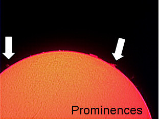
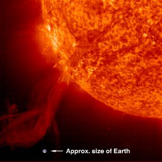
Prominences
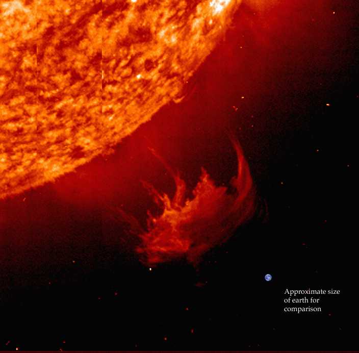
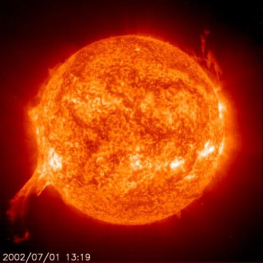
Prominences are dense clouds of material suspended above the surface of the Sun by loops of magnetic field. Prominences and filaments are actually the same thing, except that prominences are seen projecting out above the limb, or edge, of the Sun. Both filaments and prominences can remain in a quiet or quiescent state for days or weeks. However, as the magnetic loops that support them slowly change, filaments and prominences can erupt and rise off of the Sun over the course of a few minutes or hours. They are often visible during a total solar eclipse.
Spicules
Like hair energized by static electricity, thousands upon thousands of glowing tendrils reach out from the Sun. Since these “spicules” of hot gas were discovered in 1877, scientists have been scratching their heads over what causes them. New observations by three observatories coupled with powerful computer modelling appear to have now solved the mystery.
The spikes of superheated gas, called plasma, are small compared to many of the Sun’s prominent features, such as giant loops of magnetic energy that are flung many thousands of miles into the solar atmosphere. The spicules are typically 300 miles (480 km) in diameter and shoot a relatively modest 3,000 miles (4,830 km) above the Sun’s surface. They scream upward at 50,000 mph (22 kps) and then vanish within five minutes, making them hard to study. More than 100,000 spicules tickle the solar atmosphere, called the corona, at any time.
The key to their origin is in the regular cycle with which spicules regenerate. Every five minutes or so, one leaps forth from the same spot, according to a new study. It so happens that the Sun has a well-known inner ring, much like that of a bell, that works on the same cycle.
A recently developed computer model of the Sun’s atmosphere shows that the periodicity of the spicules is caused by sound waves at the solar surface that have the same five-minute period
The ringing of the Sun involves seismic waves similar to those in an earthquake. They are usually damped down before they can leave the surface and so continue bouncing around inside the Sun. They are basically sound waves that are trapped, and for the most part they can’t escape to the outside.
But the study found that some of the sound waves leak out, developing shock waves that propel matter upward to generate spicules and push them into the corona.
Scientists don’t know exactly how the mass of the solar wind gets into the corona nor what accelerates the particles into space. The spicules are a good candidate, as they carry into the atmosphere more than 100 times the mass needed to feed the solar wind.
Most of the mass of the spicules comes back down, but only a fraction would have to remain high up to account for the solar wind. However, it’s not clear how much if any of the mass from the spicules remains in the corona, or if it is heated to the extent that appears to be required to create the super energetic particles of the solar wind.
Spicules are usually associated with concentrated magnetic tubes called flux tubes, giant loops that link one region of magnetic polarity to another by arcing out from the surface and back to another spot thousands of miles away. The tubes are mostly vertical, but some are inclined away from the vertical, and that’s where the sound waves tend to leak out.
Dark features in right of image are spicules, jets of gas moving toward the camera at about 30,000 mph (13.4 kps). In upper left are small sunspots and large magnetic loops connecting the sunspots. The brighter areas are strong areas of magnetism called “plage” regions, usually organized in small flux tubes. The photo measures 40,000 miles (64,370 km) across. (Image courtesy: Royal Swedish Academy of Sciences).
Helmet Streamers
Helmet streamers are large cap-like coronal structures with long pointed peaks that usually overlie sunspots and active regions. We often find a prominence or filament lying at the base of these structures. A network of magnetic loops that connect the sunspots in active regions and help suspend the prominence material above the solar surface forms helmet streamers. The closed magnetic field lines trap the electrically charged coronal gases to form these relatively dense structures. The pointed peaks are formed by the action of the solar – wind blowing away from the Sun in the spaces between the streamers.
Polar Plumes
Polar plumes are long thin streamers that project outward from the Sun’s north and south poles. We often find bright areas at the footpoints of these features that are associated with small magnetic regions on the solar surface. These structures are associated with the “open” magnetic field lines at the Sun’s poles. The plumes are formed by the action of the solar wind in much the same way as the peaks on the helmet streamers.
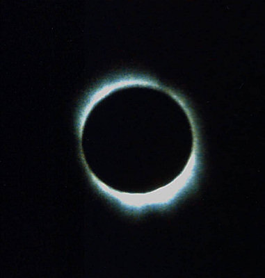
The White-Light Corona
The Corona is the Sun’s outer atmosphere. It is visible during total eclipses of the Sun as a pearly white crown surrounding the Sun. The corona displays a variety of features including streamers, plumes, and loops. These features change from eclipse to eclipse and the overall shape of the corona changes with the sunspot cycle. However, during the few fleeting minutes of totality few, if any, changes are observed in these coronal features.
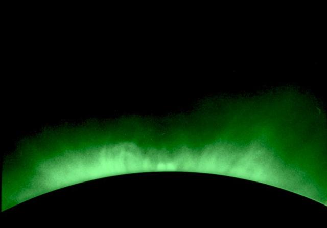
The Emission Line Corona
Early observations of the visible spectrum of the corona revealed bright emission lines at wavelengths that did not correspond to any known materials. This led astronomers to propose the existence of “coronium” as the principal gas in the corona. The true nature of the corona remained a mystery until it was determined that the coronal gases are super-heated to temperatures greater than 1,000,000ºC (1,800,000ºF). At these high temperatures both hydrogen and helium (the two dominant elements) are completely stripped of their electrons. Even minor elements like carbon, nitrogen, and oxygen are stripped down to bare nuclei. Only the heavier trace elements like iron and calcium are able to retain a few of their electrons in this intense heat. It is emission from these highly ionized elements that produces the spectral emission lines that were so mysterious to early astronomers. We can now produce artificial eclipses in coronagraphs that cover the disk of the Sun and filter out everything except the emission due to these coronal ions.
The Solar Wind
The solar wind streams off of the Sun in all directions at speeds of about 400 km/s (about 1 million miles per hour). The source of the solar wind is the Sun’s hot corona. The temperature of the corona is so high that the Sun’s gravity cannot hold on to it. Although it is understood why this happens it is not understood about how and where the coronal gases are accelerated to these high velocities. This question is related to the question of Coronal heating.
The sun is flinging 1 million tons of matter out into space every second! We call this material solar wind. But just what makes up the solar wind, how dense is it, how fast does it travel and just how hot is it?
The solar wind is made of Hydrogen (95%) and Helium (4%) and Carbon, Nitrogen, Oxygen, Neon, Magnesium, Silicon and Iron (~1%). These atoms are all in the form of positive ions which means they have lost electrons because the temperature is so hot. So really, solar wind is positive ions and the electrons these ions have lost. We call this plasma.
At the orbit of the Earth, the solar wind has an average density of about 6 ions/cm3. This is not very dense at all! So even though the solar wind moves incredibly fast (normally in the range from 300 to 600 km/s), it wouldn’t even ruffle your hair if you were to stand directly in the midst of a solar wind breeze! But, some explosive events like solar flares or CME’s on the Sun can produce speeds over 1000 km/s!
The solar wind goes all the way past Pluto. The Voyager 1 spacecraft has gone past the Termination Shock at 90AU, where the spacecraft is currently operating in the heliosheath environment which is still dominated by the Sun’s magnetic field and particles contained in the solar wind. The heliosheath exploration phase ends with passage through the heliopause which is the outer extent of the Sun’s magnetic field and solar wind. The thickness of the heliosheath is uncertain and could be tens of AU thick taking several years to traverse. Passage through the heliopause begins the interstellar exploration phase with the spacecraft operating in an interstellar wind dominated environment. This interstellar exploration is the ultimate goal of the Voyager Interstellar Mission.
The temperature of solar wind plasma around the Earth is about 150,000°K.
Solar Wind VariationsThe solar wind is not uniform. Although it is always directed away from the Sun, it changes speed and carries with it magnetic clouds, interacting regions where high-speed wind catches up with slow speed wind, and composition variations. The solar wind speed is high (800 km/s) over coronal holes and low (300 km/s) over streamers. These high and low speed streams interact with each other and alternately pass by the Earth as the Sun rotates. These wind speed variations buffet the Earth’s magnetic field and can produce storms in the Earth’s magnetosphere, the aurora.
The Ulysses spacecraft has now completed one orbit through the solar system during which it passed over the Sun’s south and north poles. Its measurements of the solar wind speed, magnetic field strength and direction, and composition have provided Solar Physicists with a new view of the solar wind.
The Advanced Composition Explorer (ACE) satellite was launched in August of 1997 and placed into an orbit about the L1 point between the Earth and the Sun. The L1 point is one of several points in space where the gravitational attraction of the Sun and Earth are equal and opposite. This particular point is located about 1.5 million km (1 million miles) from the Earth in the direction of the Sun. ACE has a number of instruments that monitor the solar wind and the spacecraft team provides real-time information on solar wind conditions at the spacecraft.
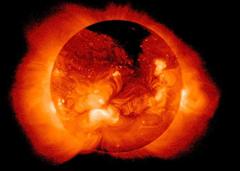
The X-Ray Corona
The corona shines brightly in x-rays because of its high temperature. On the other hand, the “cool” solar photosphere emits very few x-rays. This allows us to view the corona across the disk of the Sun when we observe the Sun in X-rays. To do this we must first design optics that can image x-rays and then we must get above the Earth’s atmosphere. In the early 70’s Skylab carried an x-ray telescope that revealed coronal holes and coronal bright points for the first time. During the last decade Yohkoh, provided a wealth of information and images on the sun’s corona. Today we have the SOHO and TRACE satellites obtaining new and exciting observations of the Sun’s corona, its features, and its dynamic character.
The “Wilson Effect”
This is an affect seen in sunspots. It was first observed in 1769 by Dr Alexander Wilson from Glasgow, who noted an unusual phenomenon in a large spot that was approaching the western limb. He followed its changing appearance and recorded the shape and proportions of its penumbra, which was first equally broad on both sides of the umbra. As the spot was carried nearer to the western limb by the Sun’s rotation he noticed that the penumbra nearer to the Sun’s centre became narrower, and when the spot was very near indeed to the limb the contracted penumbra had vanished from sight while the width of the penumbra nearest the limb remained practically unaltered. When the same spot reappeared at the east limb a fortnight or so later, he noted that the position was reversed.
Dr Wilson came to the conclusion that sunspots were in fact cavities with different depths. He explains the effect by assuming that each sunspot was a conical shape in the solar “surface” and so giving the desired effect.
The models by modern solar physicists resemble a cone. The Sun has no solid surface; it is gases with a continuously decreasing density. The umbra is more transparent than the penumbra and the penumbra is more transparent than the photosphere, the depths of the spots are 500 km’s to 1,000 km’s depending on size.
Wilson Effect Problems
Present day equipment has confirmed the Wilson effect, but a problem has arisen. The reason for this has come to light due to the limit of early optical equipment. It was also not reported by earlier observers that asymmetrical Sunspots do not show the Wilson effect, if they are very asymmetrical then it may show the complete opposite. Work done by a few solar observers has drawn to the conclusion that the shape of the spot cancels out this effect.
Coronal Loops
Coronal loops are found around sunspots and in active regions. These structures are associated with the closed magnetic field lines that connect magnetic regions on the solar surface. Many coronal loops last for days or weeks but most change quite rapidly. Some loops, however, are associated with solar flares and are visible for much shorter periods. These loops contain denser material than their surroundings. The three dimensional structure and the dynamics of these loops is an area of active research.
Coronal Holes
Coronal holes are regions where the corona is dark. These features were discovered when X-ray telescopes were first flown above the earth’s atmosphere to reveal the structure of the corona across the solar disc. Coronal holes are associated with “open” magnetic field lines and are often found at the Sun’s poles. The high-speed solar wind is known to originate in coronal holes.
Flare Characteristics
Solar flares are tremendous explosions on the surface of the Sun. In a matter of just a few minutes they heat material to many millions of degrees and release as much energy as a billion megatons of TNT. They occur near sunspots, usually along the dividing line (neutral line) between areas of oppositely directed magnetic fields.
Flares release energy in many forms – electro-magnetic (Gamma rays and X-rays), energetic particles (protons and electrons), and mass flows. Flares are characterized by their brightness in X-rays (X-Ray flux). The biggest flares are X-Class flares. M-Class flares have a tenth the energy and C-Class flares have a tenth of the X-ray flux seen in M-Class flares. The National Oceanic and Atmospheric Administration (NOAA) monitor the X-Ray flux from the Sun with detectors on some of its satellites.
Flare Observations
Solar flares are observed using filters to isolate the light emitted by hydrogen atoms in the red region of the solar spectrum (the H-alpha spectral line). Most solar observatories have H-alpha telescopes and some observatories monitor the Sun for solar flares by capturing images of the Sun every few seconds. With the introduction in the last few years of H-alpha filters affordable by amateurs, many can now carry out this work. This is very important as the energy sent out by the flares can not only cause great damage to the astronauts onboard the International Space Station, (ISS), but also disrupt electrical and radio installations on Earth, as well as giving us nice displays of aurora! These flares are normally referred to as Coronal Mass Ejections or CMEs.
Since the Sun is a ball of gas it does not have to rotate rigidly like the solid planets and moons do. In fact, the Sun’s Equatorial Regions rotate faster (taking about 24 days) than the Polar Regions (which rotate once in more than 30 days). The source of this “differential rotation” is an area of current research in solar astronomy.
NEVER LOOK AT THE SUN WITHOUT PROPER FILTRATION!